Category Archives: Finite element analysis

Vibrating window frames

Mode 1

Mode 1

Mode 2

Mode 2

Mode 3

Mode 3

Mode 4

Mode 4

Vibrating windows

Here are some nice images of vibrating window frames (ooh, wow)! The finite element model I made with Python will hopefully enable me to do two things: calculate the radiation coefficient of the window frame, and calculate the effect of coupling the wooden frame with the windowpane (although shear locking is definitely a problem for the model I’m using at the moment). These things should be very central when one considers the computational airborne sound insulation of the structure as a whole.

I’m also thinking of making a more detailed model of the music box I wrote about earlier using this model at some point. That should make a fun topic for the blog.

Simulating cymatics

Due to popular demand I put the source for the script I used here up to github: https://github.com/kai5z/Chladni-patterns

I was browsing around youtube when I stumbled upon this nice video on Chladni patterns (there are quite a few there). Here’s the video, it’s apparently part of some demonstration for students:

Cymatics

Sound propagates in solids, similarly as to how it does in air. If we were to slow down the plate in the video above, we would see it vibrating at the frequency of the sound you can hear being played (check another post of mine).

Just as is the case in air, standing waves can form in solids. In solids, the details are quite different, but the basic principle holds. When a standing wave forms, there are locations where the amplitudes of the vibrations have their maximum values, and locations where the amplitudes of the vibrations are very close to zero.

Imagine placing a lot of small particles on the surface in the image. The particles would be tossed around, until they finally find a resting place close to the red circle. This is how all of the patterns are formed, but the way the plate vibrates varies with frequency.

Simulating cymatics

The experiment setup is very clearly defined; a rectangular steel plate is clamped in the middle. This makes for a perfect case to test out some finite element analysis of plate structures!

I used steel as the material of choice for the simulation and Reissner-Mindlin bilinear plate elements, with a lumped mass matrix. I programmed the simulation using Python. By tweaking around with the material properties and dimensions, I managed to roughly match the frequencies to the experiment from the first video. I think it’s really cool how the simulation matches the patterns you can see in the video (up until a point where it’s apparent that there are some asymmetries in the setup).

I made a gif out of the video too, just for the hell of it.

You might have noticed that there are a whole lot of patterns there, which aren’t visible in the video. The standing waves which create the patterns form much more strongly when the frequency is closer to the modal frequencies of the plate (when the plate resonates). The following plot roughly shows these resonant frequencies. The y-axis doesn’t really mean anything significant here, so just pay attention to the peaks. Also, damping hasn’t been taking into account here, making the peaks unrealistically sharp. When the excitation frequency is close to one of those peaks, Chladni patterns should be clearly visible.

Discussion

The frequencies these patterns form on depends completely on the material properties and dimensions of the plate, if we assume that the basic setup is the same (a rectangular plate is clamped at the middle). There are a lot of structures which can be analysed in a similar way (albeit with a more complex analysis for applicable results): floors, windows, doors, the list goes on and on. In this case, the results were very consistent with the video as the physical problem was very clearly defined.

A tool for solving 2D structural systems

If you’re not that into structural mechanics, feel free to just look at the pictures :-). This post is about a tool that will enable you to calculate how structural systems behave in two dimensions. In the (hopefully not that distant) future, I’ll enable dynamic calculations.

I haven’t shared anything in a while, so I thought I write a status update on this cool (at least I think it is cool!) tool I’ve been working during the last few months, along with other projects. It’s based on an old idea, which I thought I’d finally realize properly. The tool is able to do finite element analysis of simple structural systems in 2D. There are quite a few things I’m planning to do differently as compared to the tools out there. For example, the tool will be able to solve symbolic problems (at least simple ones) along with numerical ones. It works quite well as long as the problem is not huge.

I was thinking of making a very early beta version of the tool available along with this post, but (as is very often the case) things have taken a bit longer than expected, and other projects have been taking up my time. So the very-early-beta release still needs some tweaking. Also, I’m not quite sure about liability issues with releasing a not-so-perfectly working version of a tool such as this, so I might never release it. We’ll see.

Overview

Some theory:

  • I’ve currently implemented basic functionality for solving structural systems consisting of beams (with axial and/or moment loads according to my previous post)
  • A linear elastic problem (static) is solved

The logic has been implemented in such a way that it should be relatively straightforward to extend the functionality to problems involving small amplitude (linear) vibrations, for examining vibrating systems in 2D. I’m really looking forward to getting to play around with that phase of the project. But, first things first, I’ve got to get static problems working properly and without any glitches.

Examples

Here are some examples of simple linear static beam structures the tool is currently able to give the correct symbolic answer to. Some background:

  • The cases have been done using a nifty GUI, which I’m quite happy with
  • L is half of the width of the figures (often the length of the beam)
  • The magnitude of the force is F
  • All cross sectional properties are given by E, I and A
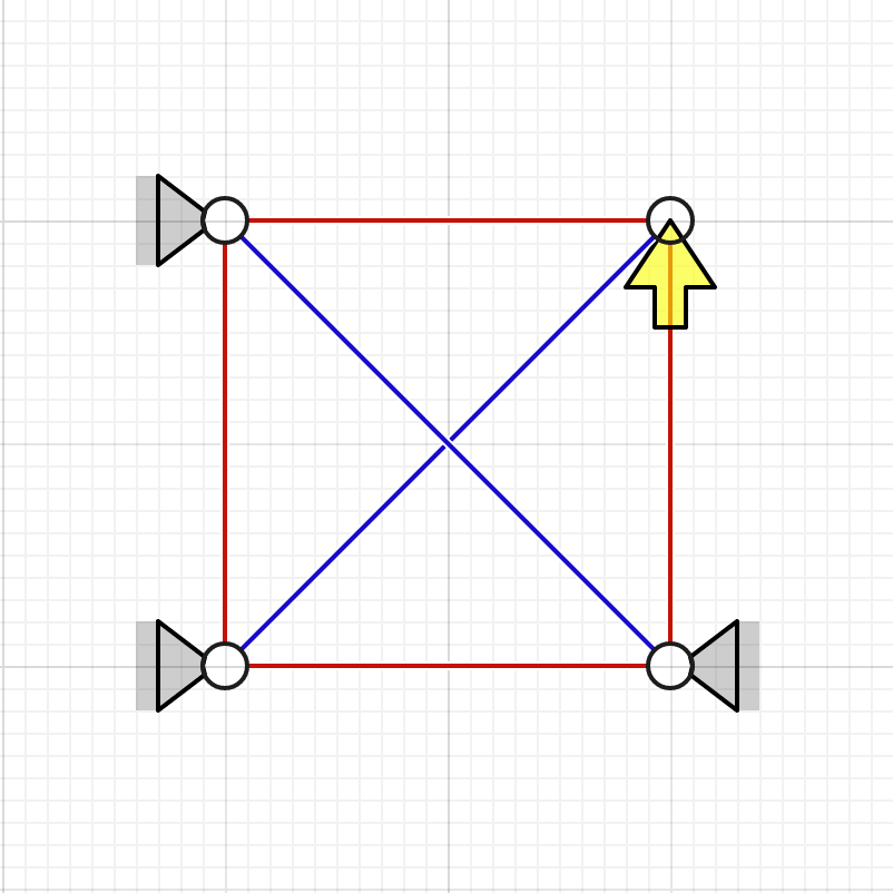
    • Except for the blue bars, which have a cross sectional area of $$2\sqrt{2}A$$
    • The connections are assumed to align with the neutral axis
  • A hollow node represents a hinged connection
  • A filled node represents a stiff connection
  • The positive x-axis points towards the right
  • The positive y-axis points downwards

The nodes are numbered from the left to the right, so just count them from the left if you want to validate the results. There are quite a few analytical formulas available for these situations if you try searching online.

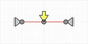
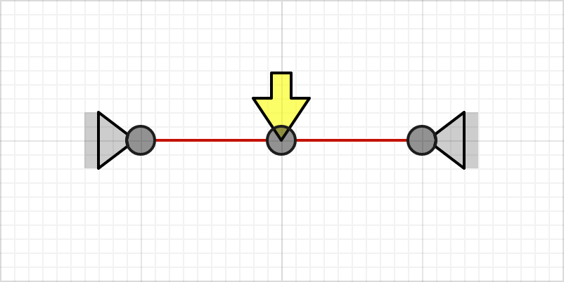
Case 1, $$\begin{Bmatrix}{}x_2\\y_2\\\theta_2\end{Bmatrix}=\begin{Bmatrix}{}0\\\frac{F L^{3}}{192 E I}\\0\end{Bmatrix}$$

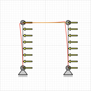
Case 2, $$\begin{Bmatrix}{}\theta_1\\a_3\\\theta_3\\x_2\\y_2\\\theta_2\end{Bmatrix}=\begin{Bmatrix}{}\frac{F L^{2}}{16 E I}\\0\\- \frac{F L^{2}}{16 E I}\\0\\\frac{F L^{3}}{48 E I}\\0\end{Bmatrix}$$

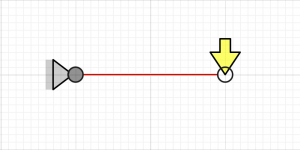
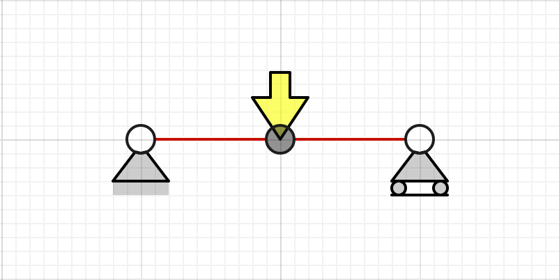
Case 3, $$\begin{Bmatrix}{}x_2\\y_2\\\theta_2\end{Bmatrix}=\begin{Bmatrix}{}0\\\frac{F L^{3}}{3 E I}\\\frac{F L^{2}}{2 E I}\end{Bmatrix}$$

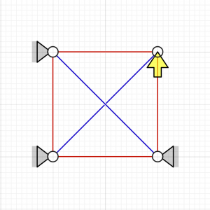
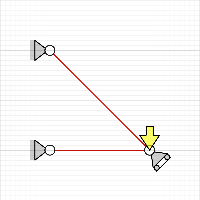
Case 4, $$\begin{Bmatrix}{x_3}\\{y_3}\end{Bmatrix}=\begin{Bmatrix}{}- \frac{F L}{3 A E}\\- \frac{2 F L}{3 A E}\end{Bmatrix}$$

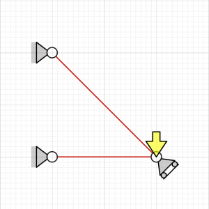
Case 5, $$a_3=\frac{\sqrt{2} F L}{A E}$$ (positive to the left)

The future

The results coincide with solutions such as these, which means that everything is working properly (woohoo)!

So far, the GUI has been the most demanding part of the project. There’s still a lot to be done. Static calculations might be something the average structural engineer finds even more useful than dynamic calculations, so those are currently my top priority. Still, the really cool stuff (in my opinion) will be possible once you’ll be able to investigate dynamic systems, which is helpful for both acoustical/vibration consultants and structural engineers alike!
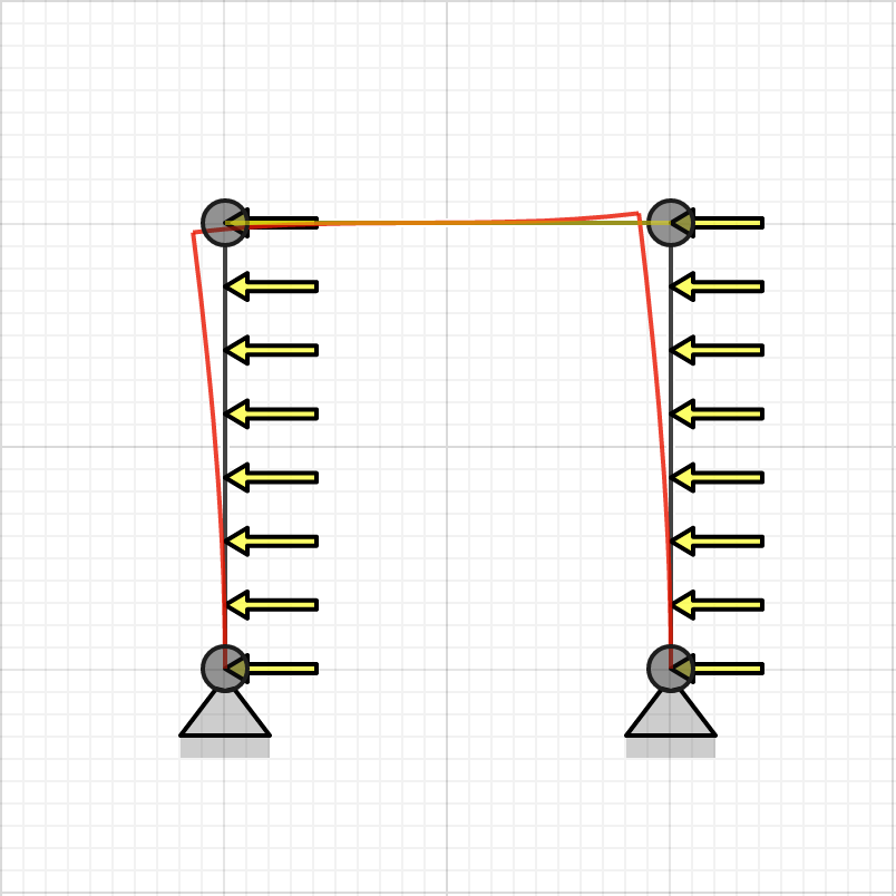
Deformed beams

Airborne sound insulation

I thought it would be cool to demonstrate some of the vary basics behind airborne sound insulation using a finite element simulation. This is also something I’m planning on utilising in real projects (i.e. it’s not just for playing around with).

Some background

Let’s assume that we have two rooms with nothing but a small piece of wall between them. The rooms are perfectly separated from each other, they’re connected by nothing but this one piece of wall. This means that the situation is analogous to laboratory measurements (i.e. when measuring the sound reduction index R, or the single-number quantity Rw). Situations on the field are different from the situation described here, as flanking transmissions are not taken into account in laboratory measurements.

Let’s also assume that this simple, homogenous piece of wall is perfectly sealed. It’s modeled as simply supported (we’re allowing for rotation on the boundaries) in 2D.

I’m not going to go any deeper into the material parameters I used here, but here’s some background on the theory:

  • The simulation is done using a Timoshenko model for the piece of wall (taking shear locking into account using reduced integration).
  • I used linear shape functions for both the fluid and beam domains.
  • The bottom boundary is completely absorbing.
  • There are two completely separate fluid domains, which are both coupled to the piece of wall in the middle.
  • I did the simulation in python, and exported the results to a binary file which is read by the javascript viewer below.

Simulation 1

http://kaistale.com/blog/131125coupling/viewer.html

The simulation is a bit heavier than in the simulations I’ve usually posted, as I had to use more elements to get a nice looking result. Here’s a very short summary of what’s happening:

  1. A sound wave travels in the lower room.
  2. The sound wave arrives at the wall.
  3. The sound wave consists of positive pressure (as compared to the surroundings and other side of the wall), and will as such exert forces on the wall.
  4. The wall will deform as a consequence of the force. Note that the deformations of the wall are exaggerated in the visualization!
  5. As the wall deforms, it moves the air above it, creating new sound waves.

Simulation 2

I also made the following simulation, which is more complex and more difficult to understand, but looks way cooler. I especially like it that you can see the sound moving faster in the wall than in the air when the first wave hits the wall (compare the sound waves below the wall to the sound waves above the wall).

Note:  I switched the colors, here red represents a positive sound pressure. Also, the wall is clamped (rotation isn’t allowed at the ends of the wall).

http://kaistale.com/blog/131126coupling/viewer.html

Epilogue

The most important thing to note is that when you’re hearing sound through the wall, as in the simulated situations, what you’re hearing are the deformations of the wall. It’s the wall that radiates sound into the room. If the wall wouldn’t move at all as a consequence of the pressure waves hitting it, you wouldn’t hear anything. This is why heavy structures, such as concrete, isolate sounds so well.

The situation becomes a whole lot more complicated with separated structures (i.e. light structures or drywall), and when flanking is taken into account. Measuring the sound reduction index with a diffuse sound field is another interesting task I’ll definitely have to do. I’ll most likely return to these topics in later posts. 🙂